![]()
Grid Topology Generation
This notebook demonstrates how to artificially generate a power grid topology. We consider the so-called Chung-Lu-Chain graph model, and refer to Aksoy et al. (2018).
Basics
[1]:
import numpy as np
import sys
import os
import matplotlib.pyplot as plt

from powergrid_synth import (
    PowerGridGenerator,
    InputConfigurator,
    HierarchicalAnalyzer,
    GridVisualizer,
)
CLC topology generation
We consider a Chung-Lu-Chain graph model for the grid topology generation. It contains two phases:
Phase 1: For each the same-voltage subgraph, we consider the Chung-Lu-Chain model that takes as input the desired node degree sequence and the desired graph diameter.
Phase 2: After the same-voltage subgraphs are created, transformer edges between each pair of subgraphs are inserted. This takes as input the desired transformer degree of each vertex in the subgraphs of voltage \(X\) and \(Y\).
Two operation modes
Mode I: When using the CLC graph generation model, one requires desired same-voltage subgraph degrees and diameter for Phase 1, and desired transformer degrees for Phase 2. They can be easily extracted from given (realistic) power grid topology. We can refer to this as Operation mode I — one can fit the model to existing power grid graphs and create ensembles of structurally similar graphs.
Mode II: In cases where real-world grid data is completely unavailable or when users want to scale or vary the inputs, we would prefer to use ONLY artificial input. This Opertaion mode II requires users only specifying the number of vertices in each same-voltage subgraph. Then, one would need to generate the artificial degree sequences and transformer degrees in some way, e.g., statistically using some degree distributions or fitting functions.
In this mode, users are free to decide which assumptions are most appropriate for their purposes.
In this project, we consider some statistically-significant fitting functions and distributions to generate the needed input.
Inputs for the degree distributions and transformer connection distributions
[2]:
# Define 3 voltage levels
level_specs = [
    # Level 0
    {'n': 20, 'avg_k': 4.0, 'diam': 6, 'dist_type': 'dgln'},
    # Level 1
    {'n': 20, 'avg_k': 3.0, 'diam': 10, 'dist_type': 'dgln'},
    # Level 2
    {'n': 10, 'avg_k': 2.0, 'diam': 5, 'dist_type': 'dgln'}
]

connection_specs = {
    (0, 1): {'type': 'k-stars', 'c': 0.174, 'gamma': 4.15},
    (1, 2): {'type': 'k-stars', 'c': 0.15, 'gamma': 4.15}
}
Define an input configurator
It configurates the input parameters to the needed ones for the algorithm
[3]:
print("\n[1] Configuring 3-Level Hierarchy...")

# Initialize Configurator
configurator = InputConfigurator(seed=100)

# Generating Input Parameters
params = configurator.create_params(level_specs, connection_specs)
[1] Configuring 3-Level Hierarchy...
Generating Level 0: DGLN distribution (Avg=4.0)
Generating Level 1: DGLN distribution (Avg=3.0)
Generating Level 2: DGLN distribution (Avg=2.0)
Generating Transformers 0<->1: k-Stars Model
4.15
Generating Transformers 1<->2: k-Stars Model
4.15
Generate the grid topology
[4]:
gen = PowerGridGenerator(seed=100)

print("\n[2] Generating Topology...")

grid_graph = gen.generate_grid(
    degrees_by_level=params['degrees_by_level'],
    diameters_by_level=params['diameters_by_level'],
    transformer_degrees=params['transformer_degrees'],
    keep_lcc=True, # only keep the largest connected component
)
print(f"Grid Generated: {grid_graph.number_of_nodes()} nodes, {grid_graph.number_of_edges()} edges")
[2] Generating Topology...
--- Starting Generation for 3 Voltage Levels ---
Generating Level 0...
  -> Level 0 Complete. Nodes: 21, Edges: 28
Generating Level 1...
  -> Level 1 Complete. Nodes: 23, Edges: 21
Generating Level 2...
  -> Level 2 Complete. Nodes: 12, Edges: 13
Generating Transformer Connections...
  -> Connecting Level 0 <-> Level 1
  -> Connecting Level 1 <-> Level 2
Filtering for Largest Connected Component (LCC)...
  -> Kept 53 nodes (removed 3 isolated nodes)
Grid Generated: 53 nodes, 67 edges
Visualize the generated grid
[5]:
viz = GridVisualizer()
[6]:
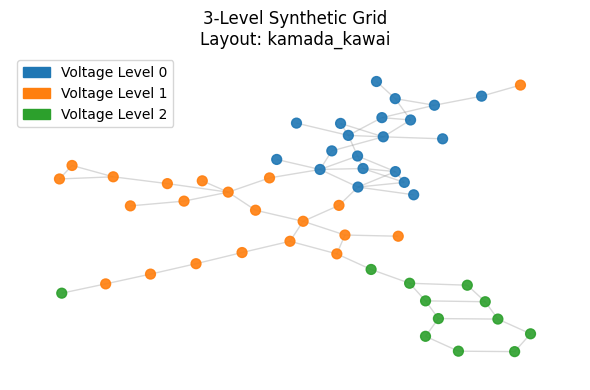
print("\n[3] Visualizing Full Grid Topology...")
viz.plot_grid(
    grid_graph,
    layout='kamada_kawai',
    title="3-Level Synthetic Grid",
    figsize=(6, 4)
)
[3] Visualizing Full Grid Topology...
Calculating layout 'kamada_kawai'...
[7]:
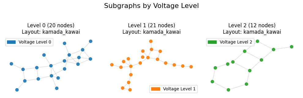
sub_lv0 = grid_graph.level(0)
sub_lv1 = grid_graph.level(1)
[8]:
print("\n[3] Visualizing Sub-Grid Topology...")
viz.plot_subgraphs(grid_graph, figsize=(10,3))
[3] Visualizing Sub-Grid Topology...
Calculating layout 'kamada_kawai'...
Calculating layout 'kamada_kawai'...
Calculating layout 'kamada_kawai'...
Analyze the generated topology
[9]:
print("\n[4] Running Hierarchical Analysis...")

# Initialize the Analyzer
analyzer = HierarchicalAnalyzer(grid_graph)

# Run the full report
# - Calculates global metrics (Diameter, Clustering, etc.)
# - Calculates metrics for EACH voltage level subgraph
# - Plots degree distributions (Log-Log scale)
analyzer.run_full_report(log_scale=True)

print("Analysis Complete.")
[4] Running Hierarchical Analysis...

========================================
GLOBAL GRID ANALYSIS
========================================

=== Power Grid Topological Analysis ===
Nodes: 53
Edges: 67
Density: 0.048621
Connected: Yes
Diameter: 18
Avg Shortest Path Length: 6.6829
Avg Local Clustering Coeff: 0.1075
=======================================

Plotting Global Degree Distribution...
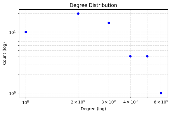
========================================
ANALYSIS FOR VOLTAGE LEVEL 0
========================================

=== Power Grid Topological Analysis ===
Nodes: 20
Edges: 28
Density: 0.147368
Connected: Yes
Diameter: 7
Avg Shortest Path Length: 3.1105
Avg Local Clustering Coeff: 0.1733
=======================================


========================================
ANALYSIS FOR VOLTAGE LEVEL 1
========================================

=== Power Grid Topological Analysis ===
Nodes: 21
Edges: 21
Density: 0.100000
Connected: No (Metrics based on LCC of size 20)
Diameter: 10
Avg Shortest Path Length: 4.1421
Avg Local Clustering Coeff: 0.1111
=======================================


========================================
ANALYSIS FOR VOLTAGE LEVEL 2
========================================

=== Power Grid Topological Analysis ===
Nodes: 12
Edges: 13
Density: 0.196970
Connected: No (Metrics based on LCC of size 11)
Diameter: 6
Avg Shortest Path Length: 2.5818
Avg Local Clustering Coeff: 0.0000
=======================================

Plotting Combined Figure for 3 Levels (Log Scale: True)...
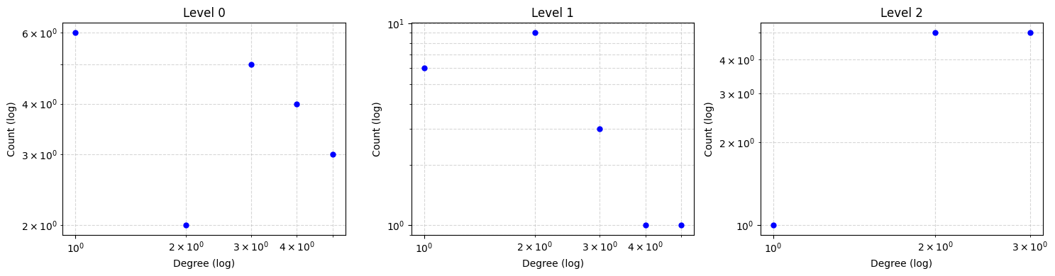
Analysis Complete.
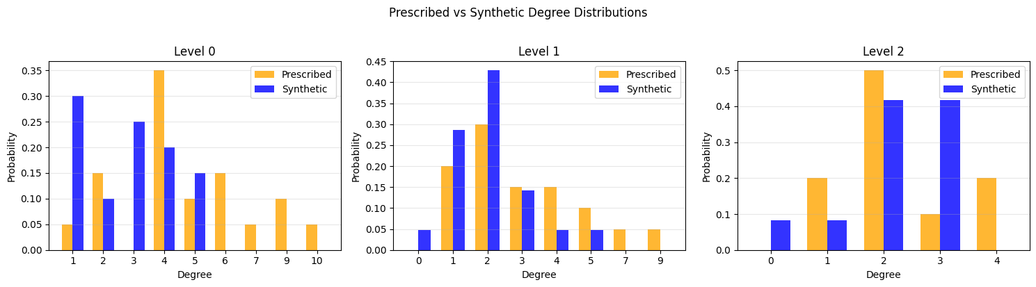
Prescribed vs synthetic degree distribution
The CLC model takes a prescribed (desired) degree sequence as input and produces a random graph whose actual degree sequence approximates it. Here we compare the two per voltage level using the KS statistic and the Relative Hausdorff (RH) distance.
[10]:
from scipy.stats import ks_2samp
from scipy.spatial.distance import directed_hausdorff
import pandas as pd

def relative_hausdorff(seq_a, seq_b):
    """1-D Relative Hausdorff distance between two degree sequences."""
    a = np.sort(seq_a).reshape(-1, 1).astype(float)
    b = np.sort(seq_b).reshape(-1, 1).astype(float)
    h = max(directed_hausdorff(a, b)[0], directed_hausdorff(b, a)[0])
    denom = max(a.max(), b.max())
    return h / denom if denom > 0 else 0.0

rows = []
for level, prescribed_degrees in enumerate(params['degrees_by_level']):
    sub = grid_graph.level(level)
    actual_degrees = [d for _, d in sub.degree()]

    ks_stat, _ = ks_2samp(prescribed_degrees, actual_degrees)
    rh = relative_hausdorff(prescribed_degrees, actual_degrees)

    rows.append({
        'Level': f'Level {level}',
        'Prescribed #nodes': len(prescribed_degrees),
        'Actual #nodes': len(actual_degrees),
        'KS Statistic': round(ks_stat, 4),
        'RH Distance': round(rh, 4),
    })

df = pd.DataFrame(rows)
print("Prescribed vs Synthetic Degree Distribution Comparison")
df
Prescribed vs Synthetic Degree Distribution Comparison
[10]:
| Level | Prescribed #nodes | Actual #nodes | KS Statistic | RH Distance | |
|---|---|---|---|---|---|
| 0 | Level 0 | 20 | 20 | 0.4500 | 0.5000 |
| 1 | Level 1 | 20 | 21 | 0.2619 | 0.4444 |
| 2 | Level 2 | 10 | 12 | 0.2000 | 0.2500 |
[11]:
from collections import Counter

n_levels = len(params['degrees_by_level'])
fig, axes = plt.subplots(1, n_levels, figsize=(5 * n_levels, 4))
if n_levels == 1:
    axes = [axes]

for level, ax in enumerate(axes):
    prescribed = params['degrees_by_level'][level]
    actual = [d for _, d in grid_graph.level(level).degree()]

    # Compute probabilities
    c_pre = Counter(prescribed)
    c_act = Counter(actual)
    all_k = sorted(set(list(c_pre.keys()) + list(c_act.keys())))

    p_pre = [c_pre.get(k, 0) / len(prescribed) for k in all_k]
    p_act = [c_act.get(k, 0) / len(actual) for k in all_k]

    width = 0.35
    x = np.arange(len(all_k))
    ax.bar(x - width/2, p_pre, width, label='Prescribed', color='orange', alpha=0.8)
    ax.bar(x + width/2, p_act, width, label='Synthetic', color='blue', alpha=0.8)
    ax.set_xticks(x)
    ax.set_xticklabels(all_k)
    ax.set_xlabel('Degree')
    ax.set_ylabel('Probability')
    ax.set_title(f'Level {level}')
    ax.legend()
    ax.grid(True, alpha=0.3, axis='y')

plt.suptitle('Prescribed vs Synthetic Degree Distributions', y=1.02)
plt.tight_layout()
plt.show()