![]()
PEGASE 9241 large-scale test
[1]:
import pandapower as pp
import pandapower.networks as pn
import pandas as pd
import numpy as np
import networkx as nx

from powergrid_synth import (
    PowerGridGenerator,
    BusTypeAllocator,
    GraphComparator,
    CapacityAllocator,
    LoadAllocator,
    GenerationDispatcher,
    TransmissionLineAllocator,
    pandapower_to_nx,
    nx_to_pandapower,
    extract_topology_params_from_graph,
)
Load the PEGASE 9241 grid using pandapower
[2]:
# 1. Load Real Grid and Convert
print("\n[1] Loading Reference Grid (PEGASE 9241)...")
net_real = pn.case9241pegase()
graph_real = pandapower_to_nx(net_real)
base_kv_list = graph_real.graph['base_kv_map']
print(f"Loaded {graph_real.number_of_nodes()} nodes and {graph_real.number_of_edges()} edges.")
[1] Loading Reference Grid (PEGASE 9241)...
Loaded 9241 nodes and 14207 edges.
Generate a synthetic grid
Extract Topology Characteristics from Graph
[3]:
print("\n[2] Analyzing Reference Topology...")
params = extract_topology_params_from_graph(graph_real)
[2] Analyzing Reference Topology...
Extracting topology parameters...
PowerGridGenerator
[4]:
# 3. Generate Synthetic Grid
print("\n[3] Generating Synthetic Clone...")
gen = PowerGridGenerator(seed=53)
synthetic_graph = gen.generate_grid(
    degrees_by_level=params['degrees_by_level'],
    diameters_by_level=params['diameters_by_level'],
    transformer_degrees=params['transformer_degrees'],
    keep_lcc=True
)
[3] Generating Synthetic Clone...
--- Starting Generation for 9 Voltage Levels ---
Generating Level 0...
  -> Level 0 Complete. Nodes: 5, Edges: 2
Generating Level 1...
  -> Level 1 Complete. Nodes: 144, Edges: 174
Generating Level 2...
  -> Level 2 Complete. Nodes: 2085, Edges: 2846
Generating Level 3...
  -> Level 3 Complete. Nodes: 4, Edges: 0
Generating Level 4...
  -> Level 4 Complete. Nodes: 3759, Edges: 4721
Generating Level 5...
  -> Level 5 Complete. Nodes: 838, Edges: 1013
Generating Level 6...
  -> Level 6 Complete. Nodes: 1854, Edges: 2031
Generating Level 7...
  -> Level 7 Complete. Nodes: 14, Edges: 3
Generating Level 8...
  -> Level 8 Complete. Nodes: 2077, Edges: 2555
Generating Transformer Connections...
  -> Connecting Level 0 <-> Level 2
  -> Connecting Level 0 <-> Level 3
  -> Connecting Level 1 <-> Level 2
  -> Connecting Level 1 <-> Level 5
  -> Connecting Level 2 <-> Level 3
  -> Connecting Level 2 <-> Level 4
  -> Connecting Level 2 <-> Level 6
  -> Connecting Level 2 <-> Level 7
  -> Connecting Level 2 <-> Level 8
  -> Connecting Level 3 <-> Level 4
  -> Connecting Level 4 <-> Level 6
  -> Connecting Level 4 <-> Level 7
  -> Connecting Level 4 <-> Level 8
  -> Connecting Level 6 <-> Level 8
Filtering for Largest Connected Component (LCC)...
  -> Kept 9282 nodes (removed 1498 isolated nodes)
Analysis
[5]:
# 5. Compare using the Library Module
print("\n[5] Running Comparative Analysis...")
comparator = GraphComparator(
    synth_graph=synthetic_graph,
    ref_graph=graph_real,
    synth_label="Synthetic",
    ref_label="PEGASE 9241"
)
[5] Running Comparative Analysis...
[6]:
comparator.plot_degree_comparison(log_scale=True, fig_size=(6,4), show_lines=True,)
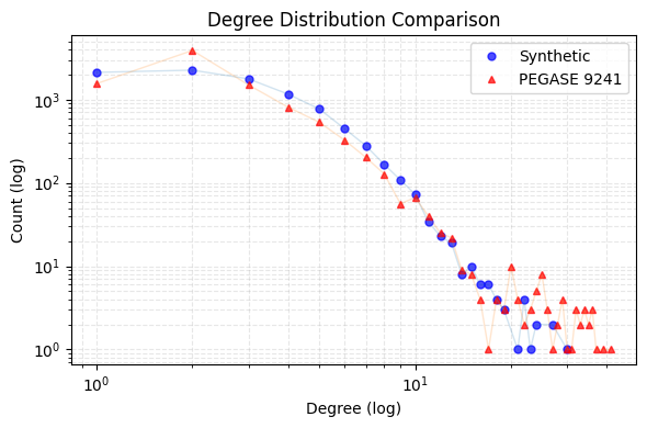
[7]:
comparator.print_level_metrics()
============================================================
LEVEL 0 COMPARISON
============================================================
            Metric Synthetic PEGASE 9241
             Nodes         1           3
             Edges         0           2
           Density  0.000000    0.666667
        Connected?       Yes         Yes
    Diameter (LCC)         0           2
Avg Path Len (LCC)    0.0000      1.3333
    Avg Clustering    0.0000      0.0000
      Transitivity    0.0000      0.0000
============================================================


============================================================
LEVEL 1 COMPARISON
============================================================
            Metric Synthetic PEGASE 9241
             Nodes       135         126
             Edges       174         174
           Density  0.019237    0.022095
        Connected?        No         Yes
    Diameter (LCC)        19          17
Avg Path Len (LCC)    7.4254      6.8424
    Avg Clustering    0.1246      0.0789
      Transitivity    0.1392      0.0845
============================================================


============================================================
LEVEL 2 COMPARISON
============================================================
            Metric Synthetic PEGASE 9241
             Nodes      1911        1814
             Edges      2842        2706
           Density  0.001557    0.001646
        Connected?        No          No
    Diameter (LCC)        77          73
Avg Path Len (LCC)   26.8720     24.5088
    Avg Clustering    0.1081      0.1066
      Transitivity    0.1239      0.2654
============================================================


============================================================
LEVEL 3 COMPARISON
============================================================
            Metric Synthetic PEGASE 9241
             Nodes         1           2
             Edges         0           1
           Density  0.000000    1.000000
        Connected?       Yes         Yes
    Diameter (LCC)         0           1
Avg Path Len (LCC)    0.0000      1.0000
    Avg Clustering    0.0000      0.0000
      Transitivity    0.0000      0.0000
============================================================


============================================================
LEVEL 4 COMPARISON
============================================================
            Metric Synthetic PEGASE 9241
             Nodes      3206        3185
             Edges      4683        4503
           Density  0.000912    0.000888
        Connected?        No          No
    Diameter (LCC)       129         127
Avg Path Len (LCC)   45.6479     47.7528
    Avg Clustering    0.1069      0.1236
      Transitivity    0.1174      0.4383
============================================================


============================================================
LEVEL 5 COMPARISON
============================================================
            Metric Synthetic PEGASE 9241
             Nodes       707         728
             Edges       999         939
           Density  0.004003    0.003548
        Connected?        No          No
    Diameter (LCC)        48          44
Avg Path Len (LCC)   16.9501     17.4357
    Avg Clustering    0.1033      0.1142
      Transitivity    0.1133      0.1120
============================================================


============================================================
LEVEL 6 COMPARISON
============================================================
            Metric Synthetic PEGASE 9241
             Nodes      1491        1530
             Edges      2004        1803
           Density  0.001804    0.001541
        Connected?        No          No
    Diameter (LCC)        82          78
Avg Path Len (LCC)   28.5089     25.8628
    Avg Clustering    0.0865      0.0561
      Transitivity    0.1037      0.1589
============================================================


============================================================
LEVEL 7 COMPARISON
============================================================
            Metric Synthetic PEGASE 9241
             Nodes         7          10
             Edges         2           3
           Density  0.095238    0.066667
        Connected?        No          No
    Diameter (LCC)         1           1
Avg Path Len (LCC)    1.0000      1.0000
    Avg Clustering    0.0000      0.0000
      Transitivity    0.0000      0.0000
============================================================


============================================================
LEVEL 8 COMPARISON
============================================================
            Metric Synthetic PEGASE 9241
             Nodes      1823        1843
             Edges      2530        2323
           Density  0.001523    0.001369
        Connected?        No          No
    Diameter (LCC)        39          34
Avg Path Len (LCC)   15.4623     15.0676
    Avg Clustering    0.0297      0.1030
      Transitivity    0.0368      0.0899
============================================================
[8]:
comparator.compare_degree_distributions()
=================================================================
DEGREE DISTRIBUTION COMPARISON  (KS & Relative Hausdorff)
=================================================================
  Level KS Statistic RH Distance
Level 0       1.0000      1.0000
Level 1       0.1873      0.1250
Level 2       0.0957      0.2353
Level 3       1.0000      1.0000
Level 4       0.0876      0.2000
Level 5       0.0995      0.2000
Level 6       0.1382      0.1333
Level 7       0.0286      0.0000
Level 8       0.2133      0.1667
=================================================================
Note that the large KS/RH values come from the ill-posed degree distributions on the corresponding voltage levels.
Bus type assignment
[9]:
# 4. Allocate Bus Types
print("\n[4] Allocating Bus Types via AIS...")
allocator = BusTypeAllocator(synthetic_graph, entropy_model=0, bus_type_ratio=[80,60,0])
bus_types = allocator.allocate(max_iter=50)
nx.set_node_attributes(synthetic_graph, bus_types, name="bus_type")
[4] Allocating Bus Types via AIS...
Starting Bus Type Allocation (N=9282, M=14947)...
  Target Entropy Score (W*): 1.5717, Std Dev: 0.0031
  Iter 0: Best Error = 0.132178
  Iter 10: Best Error = 0.127606
  Iter 20: Best Error = 0.125055
  Iter 30: Best Error = 0.122702
  Iter 40: Best Error = 0.120258
[10]:
from collections import Counter

counts = Counter(bus_types.values())
total = sum(counts.values())
print(f"-----> Assignment Complete:")
print(f"       Generators: {counts['Gen']} ({counts['Gen']/total:.1%})")
print(f"       Loads:      {counts['Load']} ({counts['Load']/total:.1%})")
print(f"       Connectors: {counts['Conn']} ({counts['Conn']/total:.1%})")
-----> Assignment Complete:
       Generators: 5368 (57.8%)
       Loads:      3914 (42.2%)
       Connectors: 0 (0.0%)
Generation capacities and load settings
[11]:
print("\n[6] Allocating Capacity...")
cap_allocator = CapacityAllocator(synthetic_graph)
capacities = cap_allocator.allocate()
total_cap = sum(capacities.values())
print(f"Total Generation: {total_cap:.2f} MW")
nx.set_node_attributes(synthetic_graph, capacities, name="pg_max")
[6] Allocating Capacity...
Allocating Capacity for 5368 generators.
Total System Capacity Target: 336886.73 MW using Reference System 1
Total Generation: 336886.73 MW
[12]:
# Check top 10 generators
sorted_gens = sorted(capacities.items(), key=lambda x: x[1], reverse=True)
print("\nTop 5 Generators by Capacity:")
for node, cap in sorted_gens[:5]:
    print(f"  Node {node}: {cap:.2f} MW (Degree: {synthetic_graph.degree(node)})")
Top 5 Generators by Capacity:
  Node 6692: 1701.77 MW (Degree: 4)
  Node 7595: 1682.40 MW (Degree: 4)
  Node 7059: 1630.22 MW (Degree: 4)
  Node 8270: 1628.88 MW (Degree: 4)
  Node 8099: 1622.55 MW (Degree: 4)
[13]:
print("\n[7] Allocating Loads ...")
load_allocator = LoadAllocator(synthetic_graph, ref_sys_id=1)
loads = load_allocator.allocate(loading_level='H')

nx.set_node_attributes(synthetic_graph, loads, name="pl")

total_load = sum(loads.values())
print(f"Total Load: {total_load:.2f} MW")
print(f"System Loading: {total_load/total_cap:.1%}")
[7] Allocating Loads ...
Allocating Loads for 3914 load buses.
Total System Load Target: 241698.38 MW (Level: H)
Total Load: 241698.38 MW
System Loading: 71.7%
[14]:
print("\n[8] Dispatching Generation...")
dispatcher = GenerationDispatcher(synthetic_graph, ref_sys_id=1)
dispatch = dispatcher.dispatch()
nx.set_node_attributes(synthetic_graph, dispatch, name="pg")
total_gen = sum(dispatch.values())
print(f"-> Total Power Dispatched: {total_gen:.2f} MW")
print(f"-> Generation Reserve: { total_cap - total_gen:.2f} MW")
[8] Dispatching Generation...
-> Total Power Dispatched: 138527.01 MW
-> Generation Reserve: 198359.73 MW
[15]:
print("\n[9] Allocating Transmission Lines (Impedance & Capacity)...")
trans_allocator = TransmissionLineAllocator(synthetic_graph, ref_sys_id=1)
line_caps = trans_allocator.allocate()

total_lines = len(line_caps)
avg_cap = sum(line_caps.values()) / total_lines if total_lines > 0 else 0
print(f"-> Allocated {total_lines} Lines")
print(f"-> Average Line Capacity: {avg_cap:.2f} MVA")
[9] Allocating Transmission Lines (Impedance & Capacity)...
-> Allocated 14947 Lines
-> Average Line Capacity: 347.97 MVA
Convert to pandapower network
[16]:
synthetic_net = nx_to_pandapower(synthetic_graph, base_kv_map=base_kv_list)
synthetic_net
[16]:
This pandapower network includes the following parameter tables:
   - bus (9282 elements)
   - load (3914 elements)
   - gen (5367 elements)
   - ext_grid (1 element)
   - line (13234 elements)
   - trafo (1713 elements)
[17]:
pp.rundcpp(synthetic_net)
synthetic_net
[17]:
This pandapower network includes the following parameter tables:
   - bus (9282 elements)
   - load (3914 elements)
   - gen (5367 elements)
   - ext_grid (1 element)
   - line (13234 elements)
   - trafo (1713 elements)
 and the following results tables:
   - res_bus (9282 elements)
   - res_line (13234 elements)
   - res_trafo (1713 elements)
   - res_ext_grid (1 element)
   - res_load (3914 elements)
   - res_gen (5367 elements)
Compatible with pandapower
pandapower provides Newton-Raphson AC (pp.runpp) and linear DC (pp.rundcpp) power-flow solvers, and export to JSON, Excel, SQLite, Pickle.
Note:
pp.runpp(AC) may not converge for large synthetic grids;pp.rundcpp(DC) always works. For AC power flow on large grids, use pypowsybl’srun_acsolver instead (shown below).
Compatible with PowSyBl
pypowsybl provides AC and DC load-flow solvers (run_ac, run_dc), interactive grid visualisation, and export to CGMES, XIIDM, MATPOWER, PSS/E, UCTE, AMPL, BIIDM, JIIDM.
Supported data export formats
PowerGridSynth provides a unified GridExporter class that wraps the built-in export functions of pandapower and pypowsybl, supporting 12+ industry-standard data formats out of the box.
Via |
Formats |
Methods |
|---|---|---|
pandapower |
JSON, Excel, SQLite, Pickle |
|
pypowsybl |
CGMES, XIIDM, MATPOWER, PSS/E, UCTE, AMPL, BIIDM, JIIDM |
|
[18]:
from powergrid_synth import GridExporter

exporter = GridExporter(synthetic_graph, base_kv_map=base_kv_list)

# --- pandapower-based exports ---
exporter.to_json("output/pegase9241_syn.json")

# --- pypowsybl-based exports ---
exporter.to_cgmes("output/pegase9241_syn_cgmes")
exporter.to_matpower("output/pegase9241_syn")
exporter.to_psse("output/pegase9241_syn")
exporter.to_pypowsybl("output/pegase9241_syn.xiidm", format="XIIDM")
-> pandapower JSON export: output/pegase9241_syn.json
-> pypowsybl CGMES export: output/pegase9241_syn_cgmes
-> pypowsybl MATPOWER export: output/pegase9241_syn
-> pypowsybl PSS/E export: output/pegase9241_syn
-> pypowsybl XIIDM export: output/pegase9241_syn.xiidm
[19]:
import pypowsybl as ppl
[20]:
from powergrid_synth import pandapower_to_pypowsybl
[21]:
ppl_net = pandapower_to_pypowsybl(synthetic_net)
[22]:
ppl_net
[22]:
Network(id=network, name=network, case_date=2026-04-14 11:44:49.021000+00:00, forecast_distance=0:00:00, source_format=)
[23]:
ppl.loadflow.run_ac(ppl_net)
[23]:
[ComponentResult(connected_component_num=0, synchronous_component_num=0, status=MAX_ITERATION_REACHED, status_text=Reached Newton-Raphson max iterations limit, iteration_count=16, reference_bus_id='sub_6692_0', slack_bus_results=[SlackBusResult(id='sub_6692_0', active_power_mismatch=19861584.66239525)], distributed_active_power=0.0)]