Bus Type Assignment in a Synthetic Grid

In this notebook, we demonstrate how to assign bus types to the nodes in the synthetically generated grid, e.g., using the Chung-Lu-Chain model, among other methods. Assigning bus types is a necessary step towards a more realistic power grid synthesization.

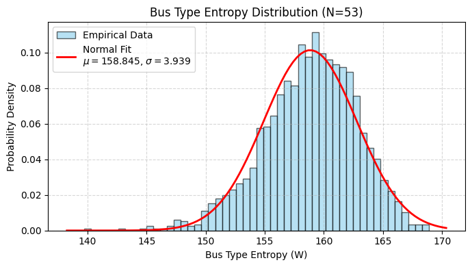
There exists a correlation between the bus types and the grid topology characteristics, which was investigated by Elyas et al. (2016). The authors also proposed a numerical measure, namely bus type entropy, to characterize this correlation and then a statistics-based method to search the best bus type assignments.

Basics

import sys
import os
import networkx as nx
from collections import Counter

from powergrid_synth import (
    PowerGridGenerator,
    InputConfigurator,
    BusTypeAllocator,
    GridVisualizer,
)

Synthetic raw topology generation

We use the previous notebook, TopologyGeneration.ipynb, for this, for three voltage levels given some limited information about the node degree distributions and the transformer connection distributions.

We refer readers to that notebook for the defined python variables.

%run TopologyGeneration.ipynb

[1] Configuring 3-Level Hierarchy...
Generating Level 0: DGLN distribution (Avg=4.0)
Generating Level 1: DGLN distribution (Avg=3.0)
Generating Level 2: DGLN distribution (Avg=2.0)
Generating Transformers 0<->1: k-Stars Model
4.15
Generating Transformers 1<->2: k-Stars Model
4.15

[2] Generating Topology...
--- Starting Generation for 3 Voltage Levels ---
Generating Level 0...
  -> Level 0 Complete. Nodes: 21, Edges: 28
Generating Level 1...
  -> Level 1 Complete. Nodes: 23, Edges: 21
Generating Level 2...
  -> Level 2 Complete. Nodes: 12, Edges: 13
Generating Transformer Connections...
  -> Connecting Level 0 <-> Level 1
  -> Connecting Level 1 <-> Level 2
Filtering for Largest Connected Component (LCC)...
  -> Kept 53 nodes (removed 3 isolated nodes)
Grid Generated: 53 nodes, 67 edges

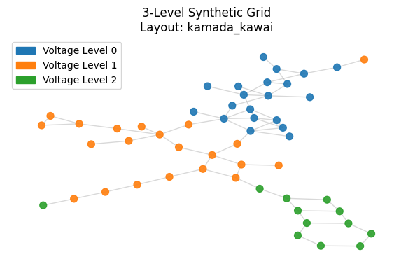
[3] Visualizing Full Grid Topology...
Calculating layout 'kamada_kawai'...

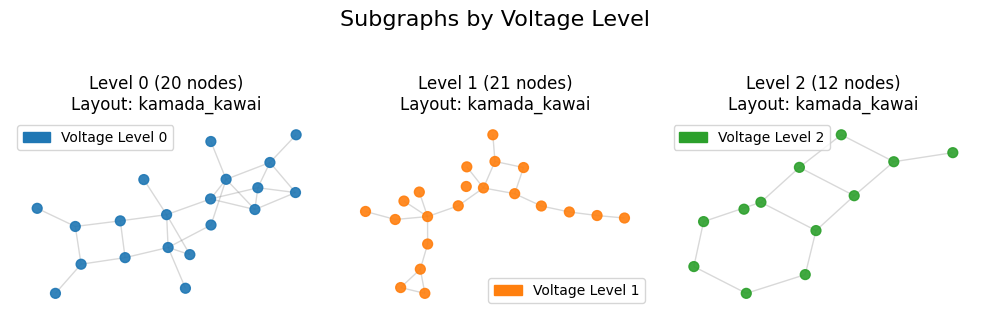
[3] Visualizing Sub-Grid Topology...
Calculating layout 'kamada_kawai'...
Calculating layout 'kamada_kawai'...
Calculating layout 'kamada_kawai'...

[4] Running Hierarchical Analysis...

========================================
GLOBAL GRID ANALYSIS
========================================

=== Power Grid Topological Analysis ===
Nodes: 53
Edges: 67
Density: 0.048621
Connected: Yes
Diameter: 18
Avg Shortest Path Length: 6.6829
Avg Local Clustering Coeff: 0.1075
=======================================

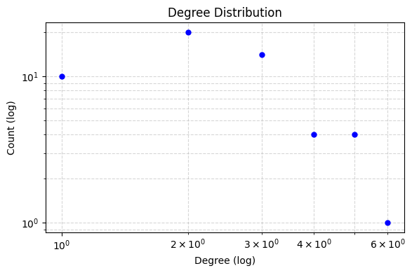
Plotting Global Degree Distribution...

========================================
ANALYSIS FOR VOLTAGE LEVEL 0
========================================

=== Power Grid Topological Analysis ===
Nodes: 20
Edges: 28
Density: 0.147368
Connected: Yes
Diameter: 7
Avg Shortest Path Length: 3.1105
Avg Local Clustering Coeff: 0.1733
=======================================


========================================
ANALYSIS FOR VOLTAGE LEVEL 1
========================================

=== Power Grid Topological Analysis ===
Nodes: 21
Edges: 21
Density: 0.100000
Connected: No (Metrics based on LCC of size 20)
Diameter: 10
Avg Shortest Path Length: 4.1421
Avg Local Clustering Coeff: 0.1111
=======================================


========================================
ANALYSIS FOR VOLTAGE LEVEL 2
========================================

=== Power Grid Topological Analysis ===
Nodes: 12
Edges: 13
Density: 0.196970
Connected: No (Metrics based on LCC of size 11)
Diameter: 6
Avg Shortest Path Length: 2.5818
Avg Local Clustering Coeff: 0.0000
=======================================

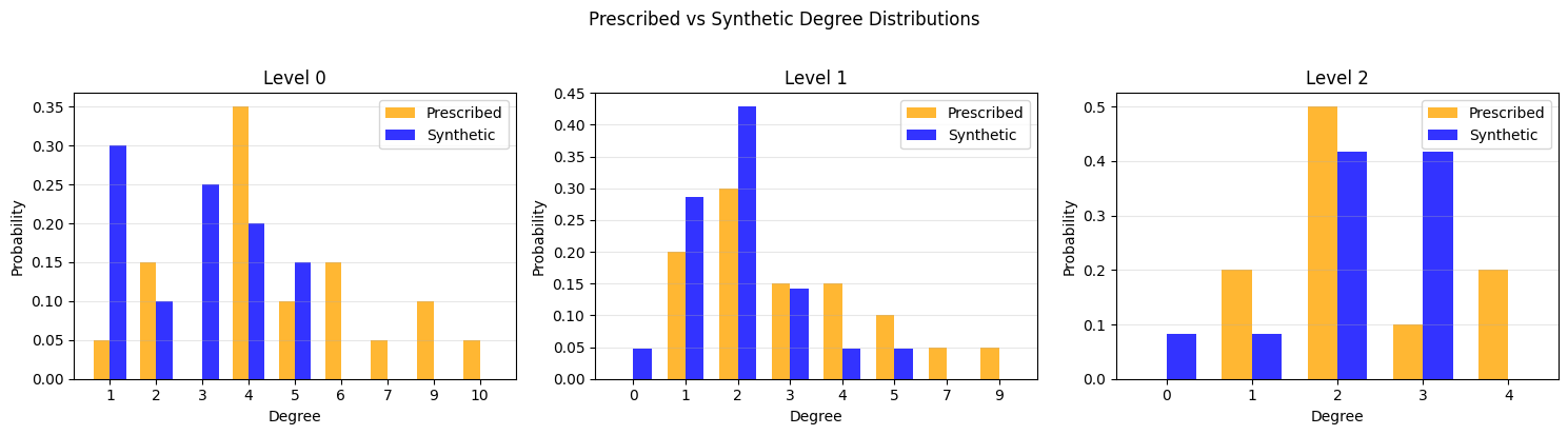
Plotting Combined Figure for 3 Levels (Log Scale: True)...

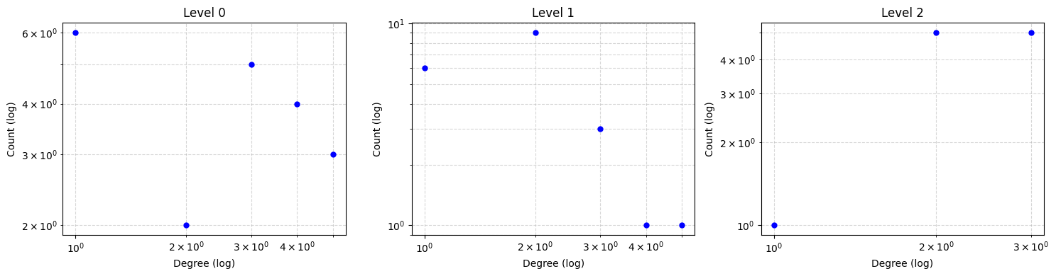
Analysis Complete.
Prescribed vs Synthetic Degree Distribution Comparison

Bus Type Assignment

allocator = BusTypeAllocator(grid_graph, entropy_model=1)
# We use a moderate iteration count for the demo
bus_types = allocator.allocate(max_iter=100, population_size=100)

Starting Bus Type Allocation (N=53, M=67)...
  Target Entropy Score (W*): 165.2889, Std Dev: 3.9391
  Iter 0: Best Error = 0.706728
  Converged at iteration 3. Error: 0.000745 < Criteria: 0.003939

allocator.plot_entropy_pdf(figsize=(7,4))

# Assign bus types as graph node attributes
nx.set_node_attributes(grid_graph, bus_types, name="bus_type")
# Show stats
counts = Counter(bus_types.values())
total = sum(counts.values())
print(f"-----> Assignment Complete:")
print(f"       Generators: {counts['Gen']} ({counts['Gen']/total:.1%})")
print(f"       Loads:      {counts['Load']} ({counts['Load']/total:.1%})")
print(f"       Connectors: {counts['Conn']} ({counts['Conn']/total:.1%})")

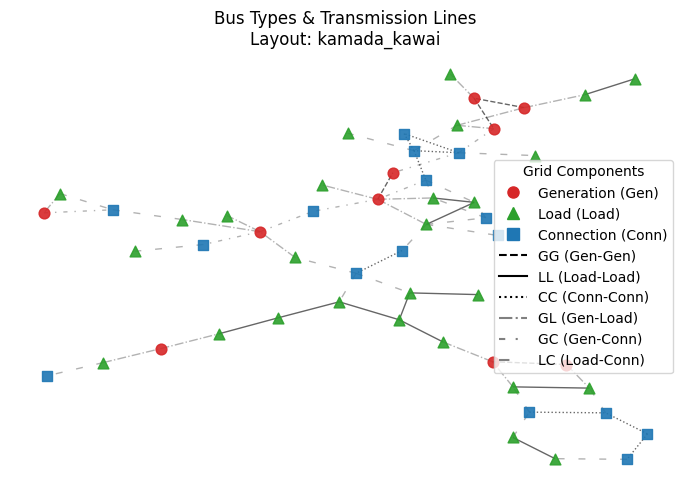
# --- 5. Bus Type Visualization ---
print("\n[5] Visualizing Bus Types & Edge Styles...")

# Call the new interactive method
viz.plot_bus_types(
    grid_graph,
    layout='kamada_kawai',
    title="Bus Types & Transmission Lines",
    figsize=(7,5)
)

-----> Assignment Complete:
       Generators: 10 (18.9%)
       Loads:      27 (50.9%)
       Connectors: 16 (30.2%)

[5] Visualizing Bus Types & Edge Styles...
Calculating layout 'kamada_kawai' for bus types...