IEEE grids for testing

[1]:

import pandapower as pp
import pandapower.networks as pn
import pandas as pd
import numpy as np
import networkx as nx
import matplotlib.pyplot as plt

from powergrid_synth import (
    PowerGridGenerator,
    BusTypeAllocator,
    GraphComparator,
    GridVisualizer,
    CapacityAllocator,
    LoadAllocator,
    GenerationDispatcher,
    TransmissionLineAllocator,
    pandapower_to_nx,
    nx_to_pandapower,
    extract_topology_params_from_graph,
)

Load an IEEE grid using pandapower

[2]:

# 1. Load Real IEEE Grid and Convert
print("\n[1] Loading Reference Grid (IEEE)...")
net_real = pn.case118()
graph_real = pandapower_to_nx(net_real)
# graph_real = create_nxgraph(net_real, respect_switches = False)
base_kv_list = graph_real.graph['base_kv_map']
print(f"Loaded {graph_real.number_of_nodes()} nodes and {graph_real.number_of_edges()} edges.")


[1] Loading Reference Grid (IEEE)...
Loaded 118 nodes and 179 edges.

[3]:

fig, ax = plt.subplots(figsize=(12,8))
ax = pp.plotting.simple_plot(net_real, ax=ax)

Generate a synthetic grid

Extract Topology Characteristics from Graph

[4]:

print("\n[2] Analyzing Reference Topology...")
params = extract_topology_params_from_graph(graph_real)

print("Extracted topology parameters:")
for key, val in params.items():
    if isinstance(val, dict):
        for k2, v2 in val.items():
            print(f"  {key}[{k2}]: {v2}")
    else:
        print(f"  {key}: {val}")


[2] Analyzing Reference Topology...
Extracting topology parameters...
Extracted topology parameters:
  degrees_by_level: [[2, 2, 2, 2, 1, 0, 0, 1, 3, 1, 2], [0, 0], [2, 2, 3, 2, 4, 2, 2, 4, 7, 2, 2, 5, 2, 5, 2, 4, 2, 2, 2, 4, 3, 2, 4, 2, 2, 3, 5, 2, 4, 2, 2, 5, 2, 4, 2, 3, 2, 2, 3, 3, 3, 2, 9, 2, 3, 2, 2, 5, 3, 5, 2, 2, 5, 3, 3, 4, 3, 2, 5, 5, 3, 2, 1, 2, 5, 2, 6, 2, 2, 6, 3, 3, 2, 5, 1, 2, 4, 2, 2, 6, 2, 5, 2, 5, 2, 2, 2, 8, 2, 2, 4, 3, 5, 3, 2, 2, 2, 4, 1, 1, 2, 2, 2, 1, 2]]
  diameters_by_level: [7, 0, 17]
  transformer_degrees[(0, 1)]: ([0, 0, 0, 0, 0, 0, 0, 0, 1, 1, 1], [3, 0])
  transformer_degrees[(0, 2)]: ([1, 0, 0, 1, 1, 1, 1, 1, 1, 1, 0], [0, 0, 0, 0, 1, 0, 0, 0, 0, 0, 0, 0, 0, 1, 0, 0, 0, 0, 0, 0, 0, 1, 0, 0, 0, 0, 0, 0, 0, 0, 0, 1, 0, 0, 0, 0, 0, 0, 0, 0, 0, 0, 0, 0, 0, 0, 0, 0, 0, 0, 0, 0, 1, 0, 1, 0, 1, 0, 0, 0, 0, 0, 0, 0, 0, 0, 0, 0, 0, 1, 0, 0, 0, 0, 0, 0, 0, 0, 0, 0, 0, 0, 0, 0, 0, 0, 0, 0, 0, 0, 0, 0, 0, 0, 0, 0, 0, 0, 0, 0, 0, 0, 0, 0, 0])
  transformer_degrees[(1, 2)]: ([1, 1], [0, 0, 0, 0, 0, 0, 0, 0, 0, 0, 0, 0, 0, 0, 0, 0, 0, 0, 0, 0, 0, 0, 0, 0, 0, 0, 0, 0, 0, 0, 0, 0, 0, 0, 0, 0, 0, 0, 0, 0, 0, 0, 0, 0, 0, 0, 0, 0, 0, 0, 0, 0, 0, 0, 0, 0, 0, 0, 1, 0, 0, 0, 0, 0, 0, 0, 0, 0, 0, 0, 0, 0, 0, 0, 1, 0, 0, 0, 0, 0, 0, 0, 0, 0, 0, 0, 0, 0, 0, 0, 0, 0, 0, 0, 0, 0, 0, 0, 0, 0, 0, 0, 0, 0, 0])

PowerGridGenerator

[5]:

# 3. Generate Synthetic Grid
print("\n[3] Generating Synthetic Clone...")
gen = PowerGridGenerator(seed=53)
synthetic_graph = gen.generate_grid(
    degrees_by_level=params['degrees_by_level'],
    diameters_by_level=params['diameters_by_level'],
    transformer_degrees=params['transformer_degrees'],
    keep_lcc=True
)


[3] Generating Synthetic Clone...
--- Starting Generation for 3 Voltage Levels ---
Generating Level 0...
  -> Level 0 Complete. Nodes: 14, Edges: 9
Generating Level 1...
  -> Level 1 Complete. Nodes: 2, Edges: 0
Generating Level 2...
  -> Level 2 Complete. Nodes: 117, Edges: 143
Generating Transformer Connections...
  -> Connecting Level 0 <-> Level 1
  -> Connecting Level 0 <-> Level 2
  -> Connecting Level 1 <-> Level 2
Filtering for Largest Connected Component (LCC)...
  -> Kept 118 nodes (removed 15 isolated nodes)

Analysis & Comparisons

[6]:

#5. Compare using the Library Module
print("\n[5] Running Comparative Analysis...")
comparator = GraphComparator(
    synth_graph=synthetic_graph,
    ref_graph=graph_real,
    synth_label="Synthetic",
    ref_label="IEEE grid"
)


[5] Running Comparative Analysis...

Compare some metric Globally

[7]:

comparator.print_metric_comparison(title="GLOBAL TOPOLOGY COMPARISON")


============================================================
GLOBAL TOPOLOGY COMPARISON
============================================================
            Metric Synthetic IEEE grid
             Nodes       118       118
             Edges       164       179
           Density  0.023758  0.025931
        Connected?       Yes       Yes
    Diameter (LCC)        14        14
Avg Path Len (LCC)    6.3178    6.3087
    Avg Clustering    0.1350    0.1651
      Transitivity    0.1146    0.1356
============================================================

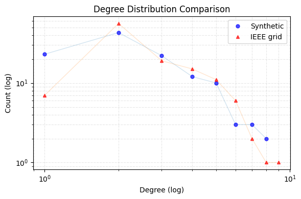
Plot the global node degree distribution for two grids

[8]:

comparator.plot_degree_comparison(log_scale=True, fig_size=(6,4), show_lines=True,)

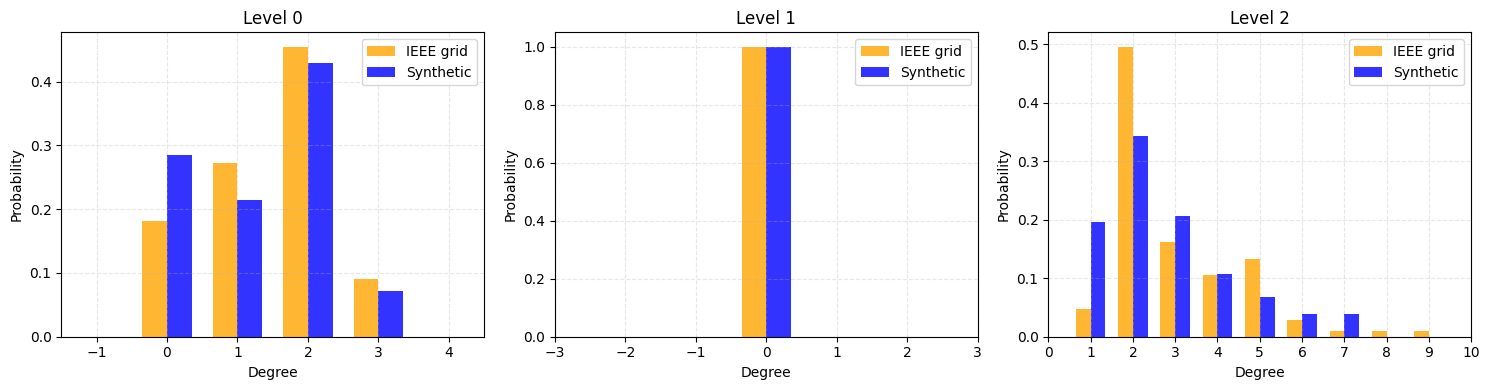
Compare the histograms of node degrees for each voltage level

[9]:

comparator.plot_all_levels_comparison(False)

Plotting Combined Comparison Figure for 3 Levels (Log Scale: False)...

Compare other topology metrics per voltage level

[10]:

comparator.plot_level_topology_comparison()

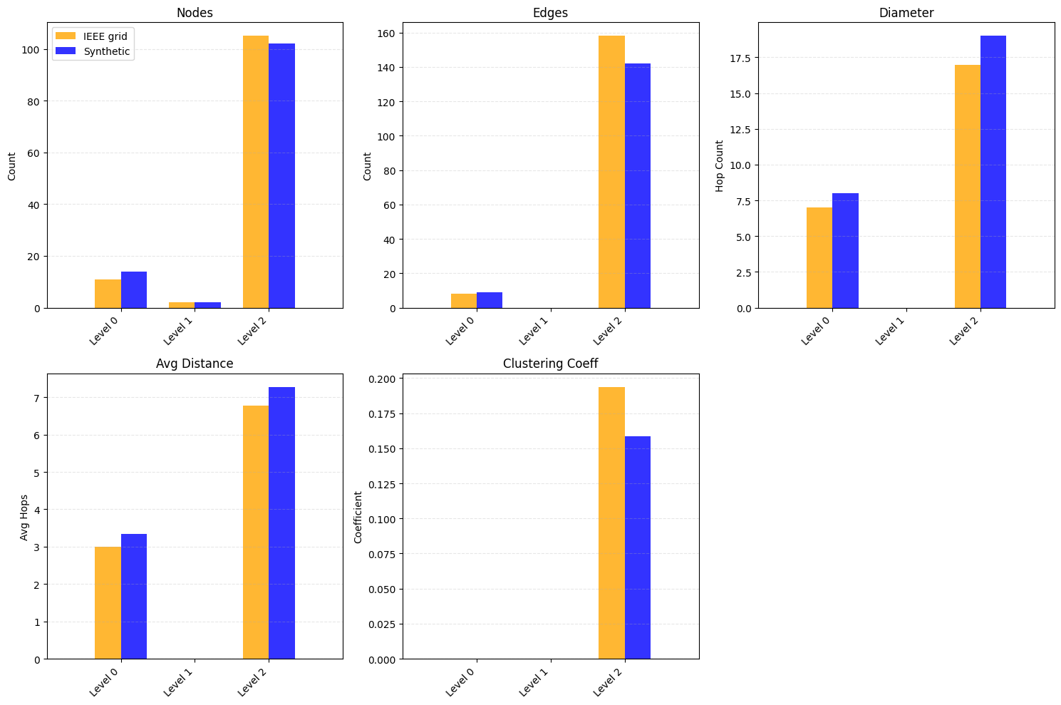
[11]:

comparator.print_level_metrics()


============================================================
LEVEL 0 COMPARISON
============================================================
            Metric Synthetic IEEE grid
             Nodes        14        11
             Edges         9         8
           Density  0.098901  0.145455
        Connected?        No        No
    Diameter (LCC)         8         7
Avg Path Len (LCC)    3.3333    3.0000
    Avg Clustering    0.0000    0.0000
      Transitivity    0.0000    0.0000
============================================================


============================================================
LEVEL 1 COMPARISON
============================================================
            Metric Synthetic IEEE grid
             Nodes         2         2
             Edges         0         0
           Density  0.000000  0.000000
        Connected?        No        No
    Diameter (LCC)         0         0
Avg Path Len (LCC)    0.0000    0.0000
    Avg Clustering    0.0000    0.0000
      Transitivity    0.0000    0.0000
============================================================


============================================================
LEVEL 2 COMPARISON
============================================================
            Metric Synthetic IEEE grid
             Nodes       102       105
             Edges       142       158
           Density  0.027567  0.028938
        Connected?       Yes       Yes
    Diameter (LCC)        19        17
Avg Path Len (LCC)    7.2745    6.7736
    Avg Clustering    0.1588    0.1936
      Transitivity    0.1349    0.1572
============================================================

[12]:

comparator.compare_degree_distributions()


=================================================================
DEGREE DISTRIBUTION COMPARISON  (KS & Relative Hausdorff)
=================================================================
  Level KS Statistic RH Distance
Level 0       0.1039      0.0000
Level 1       0.0000      0.0000
Level 2       0.1485      0.2222
=================================================================

The KS statistic measures the maximum difference between the cumulative degree distributions of the synthetic and reference graphs; values close to 0 (with large p-values) indicate the two distributions are statistically indistinguishable.
The Relative Hausdorff (RH) distance captures the worst-case mismatch in actual degree values, normalized by the maximum degree — low values mean the degree ranges align well across both grids.

Visualizations

[13]:

viz = GridVisualizer()

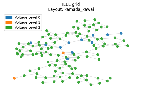
[14]:

viz.plot_grid(
    graph_real,
    layout='kamada_kawai',
    title="IEEE grid",
    figsize=(6, 4)
)

Calculating layout 'kamada_kawai'...

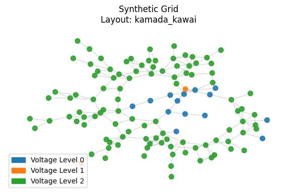
[15]:

viz.plot_grid(
    synthetic_graph,
    layout='kamada_kawai',
    title="Synthetic Grid",
    figsize=(6, 4)
)

Calculating layout 'kamada_kawai'...

Bus type assignment

[16]:

# 4. Allocate Bus Types
print("\n[4] Allocating Bus Types via AIS...")
allocator = BusTypeAllocator(synthetic_graph, entropy_model=0, bus_type_ratio=[80,60,0])
# The allocator uses the graph size to determine target ratios dynamically
bus_types = allocator.allocate(max_iter=50)
nx.set_node_attributes(synthetic_graph, bus_types, name="bus_type")


[4] Allocating Bus Types via AIS...
Starting Bus Type Allocation (N=118, M=164)...
  Target Entropy Score (W*): 1.7078, Std Dev: 0.0295
  Iter 0: Best Error = 0.000808
  Converged at iteration 1. Error: 0.000019 < Criteria: 0.000030

[17]:

from collections import Counter

counts = Counter(bus_types.values())
total = sum(counts.values())
print(f"-----> Assignment Complete:")
print(f"       Generators: {counts['Gen']} ({counts['Gen']/total:.1%})")
print(f"       Loads:      {counts['Load']} ({counts['Load']/total:.1%})")
print(f"       Connectors: {counts['Conn']} ({counts['Conn']/total:.1%})")

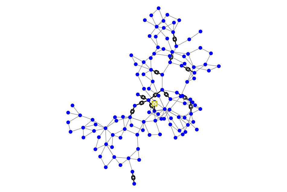
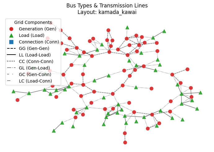
# --- 5. Bus Type Visualization ---
print("\n[5] Visualizing Bus Types & Edge Styles...")

# Call the new interactive method
viz.plot_bus_types(
    synthetic_graph,
    layout='kamada_kawai',
    title="Bus Types & Transmission Lines",
    figsize=(7,5)
)

-----> Assignment Complete:
       Generators: 66 (55.9%)
       Loads:      52 (44.1%)
       Connectors: 0 (0.0%)

[5] Visualizing Bus Types & Edge Styles...
Calculating layout 'kamada_kawai' for bus types...

Generation capacities and load settings

[18]:

print("\n[6] Allocating Capacity...")
cap_allocator = CapacityAllocator(synthetic_graph)
capacities = cap_allocator.allocate()
total_cap = sum(capacities.values())
print(f"Total Generation: {total_cap:.2f} MW")
# Attach to graph
nx.set_node_attributes(synthetic_graph, capacities, name="pg_max")


[6] Allocating Capacity...
Allocating Capacity for 66 generators.
Total System Capacity Target: 10631.90 MW using Reference System 1
Total Generation: 10631.90 MW

[19]:

# Check top 10 generators
sorted_gens = sorted(capacities.items(), key=lambda x: x[1], reverse=True)
print("\nTop 5 Generators by Capacity:")
for node, cap in sorted_gens[:5]:
    print(f"  Node {node}: {cap:.2f} MW (Degree: {synthetic_graph.degree(node)})")


Top 5 Generators by Capacity:
  Node 71: 2271.04 MW (Degree: 7)
  Node 57: 1181.96 MW (Degree: 6)
  Node 6: 392.39 MW (Degree: 1)
  Node 115: 382.98 MW (Degree: 3)
  Node 37: 333.74 MW (Degree: 5)

[20]:

print("\n[7] Allocating Loads ...")
load_allocator = LoadAllocator(synthetic_graph, ref_sys_id=1)
loads = load_allocator.allocate(loading_level='H')

# Attach to graph (attribute 'pl' for active power load)
nx.set_node_attributes(synthetic_graph, loads, name="pl")

total_load = sum(loads.values())
print(f"Total Load: {total_load:.2f} MW")

print(f"System Loading: {total_load/total_cap:.1%}")


[7] Allocating Loads ...
Allocating Loads for 52 load buses.
Total System Load Target: 8347.40 MW (Level: H)
Total Load: 8347.40 MW
System Loading: 78.5%

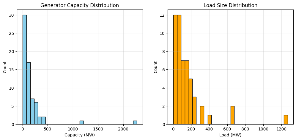
[21]:

# Plot Distribution
load_vals = list(loads.values())

if load_vals:
    plt.figure(figsize=(12, 5))

    plt.subplot(1, 2, 2)
    plt.hist(load_vals, bins=30, color='orange', edgecolor='black')
    plt.title("Load Size Distribution")
    plt.xlabel("Load (MW)")
    plt.ylabel("Count")
    plt.grid(True, alpha=0.3)

# Plot Distribution
caps = list(capacities.values())
if caps:
    plt.subplot(1, 2, 1)
    plt.hist(caps, bins=30, color='skyblue', edgecolor='black')
    plt.title("Generator Capacity Distribution")
    plt.xlabel("Capacity (MW)")
    plt.ylabel("Count")
    plt.grid(True, alpha=0.3)
    plt.show()

[22]:

print("\n[8] Dispatching Generation...")
dispatcher = GenerationDispatcher(synthetic_graph, ref_sys_id=1)
dispatch = dispatcher.dispatch()
nx.set_node_attributes(synthetic_graph, dispatch, name="pg")
total_gen = sum(dispatch.values())
print(f"-> Total Power Dispatched: {total_gen:.2f} MW")
print(f"-> Generation Reserve: { total_cap - total_gen:.2f} MW")


[8] Dispatching Generation...
-> Total Power Dispatched: 8347.40 MW
-> Generation Reserve: 2284.50 MW

[23]:

print("\n[9] Allocating Transmission Lines (Impedance & Capacity)...")
trans_allocator = TransmissionLineAllocator(synthetic_graph, ref_sys_id=1)
line_caps = trans_allocator.allocate()

total_lines = len(line_caps)
avg_cap = sum(line_caps.values()) / total_lines if total_lines > 0 else 0
print(f"-> Allocated {total_lines} Lines")
print(f"-> Average Line Capacity: {avg_cap:.2f} MVA")


[9] Allocating Transmission Lines (Impedance & Capacity)...
-> Allocated 164 Lines
-> Average Line Capacity: 1191.18 MVA

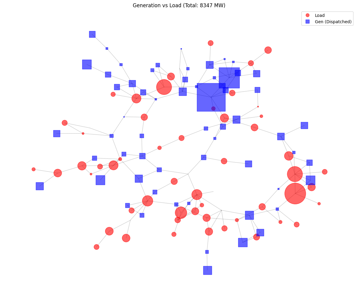
[24]:

viz = GridVisualizer()

print("-> Plotting Generation vs Load Bubbles...")
viz.plot_load_gen_bubbles(synthetic_graph, layout='kamada_kawai', title=f"Generation vs Load (Total: {total_load:.0f} MW)")

-> Plotting Generation vs Load Bubbles...

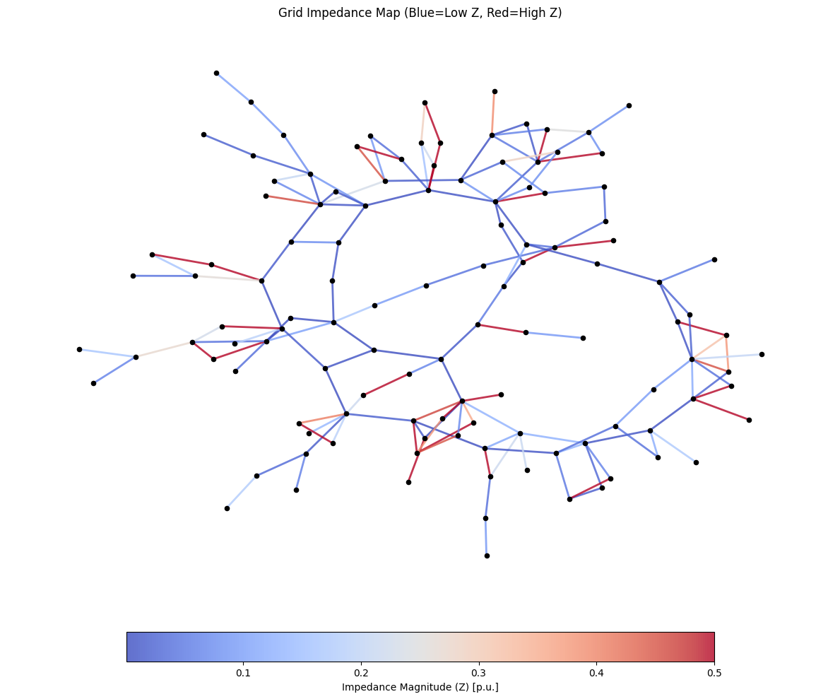
[25]:

viz.plot_impedance(synthetic_graph, layout='kamada_kawai', title="Grid Impedance Map (Blue=Low Z, Red=High Z)")

[26]:

synthetic_net = nx_to_pandapower(synthetic_graph, base_kv_map=base_kv_list)
synthetic_net

[26]:

This pandapower network includes the following parameter tables:
   - bus (118 elements)
   - load (52 elements)
   - gen (65 elements)
   - ext_grid (1 element)
   - line (151 elements)
   - trafo (13 elements)

[27]:

pp.runpp(net_real)
net_real

[27]:

This pandapower network includes the following parameter tables:
   - bus (118 elements)
   - load (99 elements)
   - gen (53 elements)
   - shunt (14 elements)
   - ext_grid (1 element)
   - line (173 elements)
   - trafo (13 elements)
   - poly_cost (54 elements)
 and the following results tables:
   - res_bus (118 elements)
   - res_line (173 elements)
   - res_trafo (13 elements)
   - res_ext_grid (1 element)
   - res_load (99 elements)
   - res_shunt (14 elements)
   - res_gen (53 elements)

[28]:

pp.rundcpp(synthetic_net)
synthetic_net

[28]:

This pandapower network includes the following parameter tables:
   - bus (118 elements)
   - load (52 elements)
   - gen (65 elements)
   - ext_grid (1 element)
   - line (151 elements)
   - trafo (13 elements)
 and the following results tables:
   - res_bus (118 elements)
   - res_line (151 elements)
   - res_trafo (13 elements)
   - res_ext_grid (1 element)
   - res_load (52 elements)
   - res_gen (65 elements)

Compatible with pandapower

pandapower provides Newton-Raphson AC (pp.runpp) and linear DC (pp.rundcpp) power-flow solvers, and export to JSON, Excel, SQLite, Pickle.

Note: pp.runpp (AC) may not converge for large synthetic grids; pp.rundcpp (DC) always works. For AC power flow on large grids, use pypowsybl’s run_ac solver instead (shown below).

[29]:

pp.runpp(synthetic_net)

[30]:

net_real.bus

[30]:

	name	vn_kv	type	zone	in_service	max_vm_pu	min_vm_pu	geo
0	1	138.0	b	1.0	True	1.06	0.94	{"coordinates": [-2.2753708781, 2.8543413351],...
1	2	138.0	b	1.0	True	1.06	0.94	{"coordinates": [-2.9368186836, 2.2121792656],...
2	3	138.0	b	1.0	True	1.06	0.94	{"coordinates": [-1.8344312496, 1.7094451782],...
3	4	138.0	b	1.0	True	1.06	0.94	{"coordinates": [-0.8886268958, 1.5532705585],...
4	5	138.0	b	1.0	True	1.06	0.94	{"coordinates": [-0.9632829393, 0.694729907], ...
...	...	...	...	...	...	...	...	...
113	114	138.0	b	1.0	True	1.06	0.94	{"coordinates": [2.2630604919, -2.7868829987],...
114	115	138.0	b	1.0	True	1.06	0.94	{"coordinates": [3.1644478736, -2.3853607175],...
115	116	345.0	b	1.0	True	1.06	0.94	{"coordinates": [-4.1528539003, -4.9348933434]...
116	117	138.0	b	1.0	True	1.06	0.94	{"coordinates": [-3.5172125372, 1.7774067282],...
117	118	138.0	b	1.0	True	1.06	0.94	{"coordinates": [-2.1457808291, -8.5466991795]...

118 rows × 8 columns

Underlying pandapower built-in export (JSON example)

[31]:

pp.to_json(net_real, filename='output/ieee118_syn.json')

Compatible with PowSyBl

pypowsybl provides AC and DC load-flow solvers (run_ac, run_dc), interactive grid visualisation, and export to CGMES, XIIDM, MATPOWER, PSS/E, UCTE, AMPL, BIIDM, JIIDM.

Supported data export formats

PowerGridSynth provides a unified GridExporter class that wraps the built-in export functions of pandapower and pypowsybl, supporting 12+ industry-standard data formats out of the box.

Via	Formats	Methods
pandapower	JSON, Excel, SQLite, Pickle	`to_json()`, `to_excel()`, `to_sqlite()`, `to_pickle()`
pypowsybl	CGMES, XIIDM, MATPOWER, PSS/E, UCTE, AMPL, BIIDM, JIIDM	`to_cgmes()`, `to_matpower()`, `to_psse()`, `to_pypowsybl(format=...)`

[32]:

from powergrid_synth import GridExporter

exporter = GridExporter(synthetic_graph, base_kv_map=base_kv_list)

# --- pandapower-based exports ---
exporter.to_json("output/ieee118_syn.json")
# exporter.to_excel("output/ieee118_syn.xlsx")
# exporter.to_sqlite("output/ieee118_syn.sqlite")
# exporter.to_pickle("output/ieee118_syn.p")

# --- pypowsybl-based exports ---
exporter.to_cgmes("output/ieee118_syn_cgmes")
exporter.to_matpower("output/ieee118_syn")
exporter.to_psse("output/ieee118_syn")
exporter.to_pypowsybl("output/ieee118_syn.xiidm", format="XIIDM")

-> pandapower JSON export: output/ieee118_syn.json
-> pypowsybl CGMES export: output/ieee118_syn_cgmes
-> pypowsybl MATPOWER export: output/ieee118_syn
-> pypowsybl PSS/E export: output/ieee118_syn
-> pypowsybl XIIDM export: output/ieee118_syn.xiidm

[33]:

import pypowsybl as ppl

[34]:

from powergrid_synth import pandapower_to_pypowsybl

[35]:

ppl_net = pandapower_to_pypowsybl(synthetic_net)

[36]:

ppl_net

[36]:

Network(id=network, name=network, case_date=2026-05-06 12:14:36.090000+00:00, forecast_distance=0:00:00, source_format=)

[37]:

ppl.loadflow.run_ac(ppl_net)

[37]:

[ComponentResult(connected_component_num=0, synchronous_component_num=0, status=CONVERGED, status_text=Converged, iteration_count=16, reference_bus_id='sub_71_0', slack_bus_results=[SlackBusResult(id='sub_71_0', active_power_mismatch=3.2199471533544965e-05)], distributed_active_power=2495.652198841721)]

Interactive grid visualizer from PowSyBl

[38]:

from pypowsybl_jupyter import network_explorer, nad_explorer, display_nad

Running the cell below, you will get to use ‘nad_explorer’ by ‘pypowsybl_jupter’ which provides an interactive visualization of the synthetic grid. Something line below

[39]:

nad_explorer(ppl_net, depth=3)

[39]:

Save the network area diagram using PowSyBl

[40]:

ppl_net.write_network_area_diagram_svg('output/ieee118_syn.svg')

[41]:

ppl_net.get_network_area_diagram()

[41]:

Underlying pypowsybl built-in export formats

[42]:

ppl.network.get_export_formats()

[42]:

['AMPL', 'BIIDM', 'CGMES', 'JIIDM', 'MATPOWER', 'PSS/E', 'UCTE', 'XIIDM']

[43]:

ppl_net.save('output/ieee118_syn.cgmes')
# or ppl_net.save('ieee118_syn', format='CGMES')