![]()
Generation Capacities and Load Settings
In previous two notebooks, we saw how the raw grid topology and the bus types can be synthetically generated.
In this notebook, we move futher in the synthetic power grid data generation by looking into how to generate capacity values for generator buses and assign load values for load buses.
Basics
[1]:
import sys
import os
import networkx as nx
from collections import Counter

from powergrid_synth import (
    PowerGridGenerator,
    InputConfigurator,
    BusTypeAllocator,
    CapacityAllocator,
    LoadAllocator,
    GenerationDispatcher,
    TransmissionLineAllocator,
    GridVisualizer,
)
Synthetic raw topology generation & Bus Type Assignment
We use the previous notebook, BusTypeAssignment.ipynb, for this.
We refer readers to that notebook for the defined python variables.
[2]:
%run BusTypeAssignment.ipynb
[1] Configuring 3-Level Hierarchy...
Generating Level 0: DGLN distribution (Avg=4.0)
Generating Level 1: DGLN distribution (Avg=3.0)
Generating Level 2: DGLN distribution (Avg=2.0)
Generating Transformers 0<->1: k-Stars Model
4.15
Generating Transformers 1<->2: k-Stars Model
4.15
[2] Generating Topology...
--- Starting Generation for 3 Voltage Levels ---
Generating Level 0...
-> Level 0 Complete. Nodes: 21, Edges: 28
Generating Level 1...
-> Level 1 Complete. Nodes: 23, Edges: 21
Generating Level 2...
-> Level 2 Complete. Nodes: 12, Edges: 13
Generating Transformer Connections...
-> Connecting Level 0 <-> Level 1
-> Connecting Level 1 <-> Level 2
Filtering for Largest Connected Component (LCC)...
-> Kept 53 nodes (removed 3 isolated nodes)
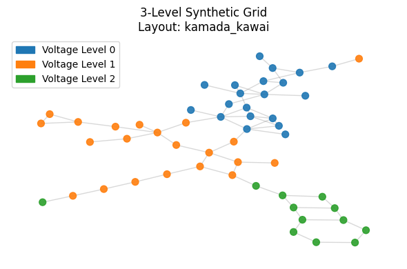
Grid Generated: 53 nodes, 67 edges
[3] Visualizing Full Grid Topology...
Calculating layout 'kamada_kawai'...
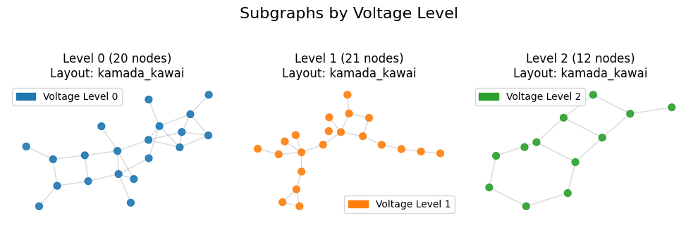
[3] Visualizing Sub-Grid Topology...
Calculating layout 'kamada_kawai'...
Calculating layout 'kamada_kawai'...
Calculating layout 'kamada_kawai'...
[4] Running Hierarchical Analysis...
========================================
GLOBAL GRID ANALYSIS
========================================
=== Power Grid Topological Analysis ===
Nodes: 53
Edges: 67
Density: 0.048621
Connected: Yes
Diameter: 18
Avg Shortest Path Length: 6.6829
Avg Local Clustering Coeff: 0.1075
=======================================
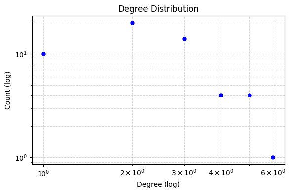
Plotting Global Degree Distribution...
========================================
ANALYSIS FOR VOLTAGE LEVEL 0
========================================

=== Power Grid Topological Analysis ===
Nodes: 20
Edges: 28
Density: 0.147368
Connected: Yes
Diameter: 7
Avg Shortest Path Length: 3.1105
Avg Local Clustering Coeff: 0.1733
=======================================


========================================
ANALYSIS FOR VOLTAGE LEVEL 1
========================================

=== Power Grid Topological Analysis ===
Nodes: 21
Edges: 21
Density: 0.100000
Connected: No (Metrics based on LCC of size 20)
Diameter: 10
Avg Shortest Path Length: 4.1421
Avg Local Clustering Coeff: 0.1111
=======================================


========================================
ANALYSIS FOR VOLTAGE LEVEL 2
========================================

=== Power Grid Topological Analysis ===
Nodes: 12
Edges: 13
Density: 0.196970
Connected: No (Metrics based on LCC of size 11)
Diameter: 6
Avg Shortest Path Length: 2.5818
Avg Local Clustering Coeff: 0.0000
=======================================

Plotting Combined Figure for 3 Levels (Log Scale: True)...
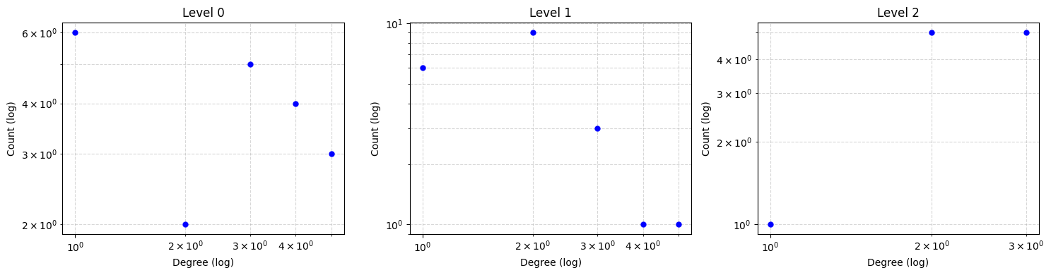
Analysis Complete.
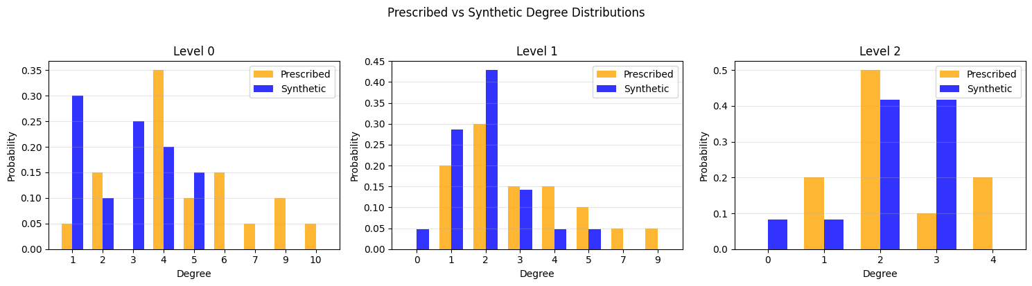
Prescribed vs Synthetic Degree Distribution Comparison
Starting Bus Type Allocation (N=53, M=67)...
  Target Entropy Score (W*): 165.2889, Std Dev: 3.9391
  Iter 0: Best Error = 0.706728
  Converged at iteration 3. Error: 0.000745 < Criteria: 0.003939
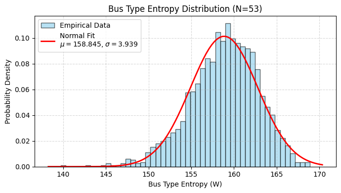
-----> Assignment Complete:
Generators: 10 (18.9%)
Loads: 27 (50.9%)
Connectors: 16 (30.2%)
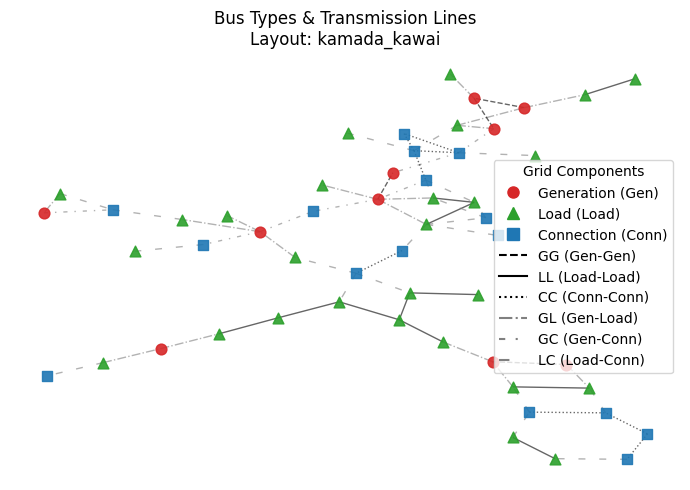
[5] Visualizing Bus Types & Edge Styles...
Calculating layout 'kamada_kawai' for bus types...
Generation Capacities
[3]:
print("\n[6] Allocating Capacity...")
cap_allocator = CapacityAllocator(grid_graph)
capacities = cap_allocator.allocate()
total_gen = sum(capacities.values())
print(f"Total Generation: {total_gen:.2f} MW")
# Attach to graph
nx.set_node_attributes(grid_graph, capacities, name="pg_max")
[6] Allocating Capacity...
Allocating Capacity for 10 generators.
Total System Capacity Target: 3869.47 MW using Reference System 1
Total Generation: 3869.47 MW
[4]:
# Check top 10 generators
sorted_gens = sorted(capacities.items(), key=lambda x: x[1], reverse=True)
print("\nTop 5 Generators by Capacity:")
for node, cap in sorted_gens[:10]:
    print(f"  Node {node}: {cap:.2f} MW (Degree: {grid_graph.degree(node)})")
Top 5 Generators by Capacity:
  Node 15: 1585.25 MW (Degree: 2)
  Node 39: 731.31 MW (Degree: 2)
  Node 9: 515.33 MW (Degree: 3)
  Node 46: 304.57 MW (Degree: 2)
  Node 2: 236.75 MW (Degree: 6)
  Node 4: 187.46 MW (Degree: 3)
  Node 20: 181.71 MW (Degree: 5)
  Node 7: 66.52 MW (Degree: 3)
  Node 38: 41.35 MW (Degree: 2)
  Node 48: 19.22 MW (Degree: 3)
Load Settings
[5]:
print("\n[7] Allocating Loads ...")
load_allocator = LoadAllocator(grid_graph, ref_sys_id=1)
loads = load_allocator.allocate(loading_level='H')

# Attach to graph (attribute 'pl' for active power load)
nx.set_node_attributes(grid_graph, loads, name="pl")

total_load = sum(loads.values())
print(f"Total Load: {total_load:.2f} MW")

print(f"System Loading: {total_load/total_gen:.1%}")
[7] Allocating Loads ...
Allocating Loads for 27 load buses.
Total System Load Target: 2806.35 MW (Level: H)
Total Load: 2806.35 MW
System Loading: 72.5%
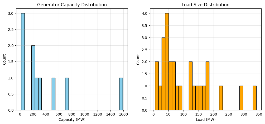
[6]:
# Plot Distribution
load_vals = list(loads.values())

if load_vals:
    plt.figure(figsize=(12, 5))

    plt.subplot(1, 2, 2)
    plt.hist(load_vals, bins=30, color='orange', edgecolor='black')
    plt.title("Load Size Distribution")
    plt.xlabel("Load (MW)")
    plt.ylabel("Count")
    plt.grid(True, alpha=0.3)

# Plot Distribution
caps = list(capacities.values())
if caps:
    plt.subplot(1, 2, 1)
    plt.hist(caps, bins=30, color='skyblue', edgecolor='black')
    plt.title("Generator Capacity Distribution")
    plt.xlabel("Capacity (MW)")
    plt.ylabel("Count")
    plt.grid(True, alpha=0.3)
    plt.show()